Chlorophyll Fluorescence measuring methods: OJIP

Chlorophyll fluorescence is one of the most popular technologies for fast non-invasive measurements of photosynthetic efficiency, which is used to get a better understanding of plants and how they react to their environment. It is very useful for quickly screening plants, like when breeding for a new cultivar, or testing the effect of a new product. Also in high-tech greenhouses, direct feedback from plants proves to be crucial for steering the climate and lighting. Other fields are also increasingly implementing chlorophyll fluorescence technologies, such as ecology, forestry and arable farming, using drones and satellites (making use of solar-induced fluorescence: SIF).

The CF2GO and PlantExplorer systems from PhenoVation measure chlorophyll fluorescence via the PAM or OJIP protocol. With PAM, we measure two distinct states of chlorophyll fluorescence during the protocol: minimum and maximum fluorescence. To do this, modulated measuring light pulses are given to the plants to obtain fluorescence signal (see the in-depth blog on the PAM protocol for more information). The difference between minimum and maximum fluorescence gives a measure of how efficiently the plant transforms light energy into chemical energy.

The OJIP protocol also measures minimum and maximum fluorescence, but zooms in specifically on this rise to maximum. In literature, this is called ‘Kautsky Chlorophyll Fluorescence Induction Kinetics’. The rise might seem simple, but it carries a surprising amount of information about how the plant is functioning and processing energy, which has been studied thoroughly over the past century by fundamental scientists.

One particularly influential model explaining the Kautsky effect was developed by Strasser and his colleagues (Strasser et al., 1995), forming the foundation of the OJIP protocol. The OJIP protocol is also deployed in the CF2GO systems, and I have briefly touched upon it in a previous blog. However, since many important and sensitive parameters are derived from OJIP, and given its complexity, I’ve decided to dedicate a full post to it. Here, I will dive into this theoretical model from Strasser. In a second part, I will go into the measured parameters. 

The OJIP rise according to Strasser

During the OJIP measurement, an extremely high-light flash is given to the plants for 1 second. A camera with a specialized sensor (highly sensitive since fluorescence is a weak signal) and filter, captures the fluorescence rise coming from the plant. 

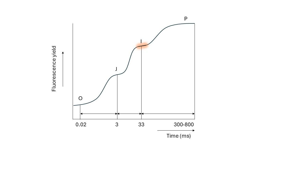
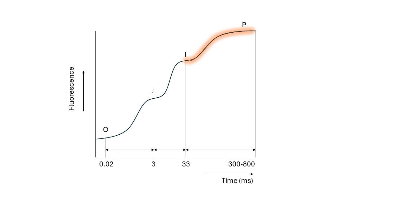
This rise does not go up in a linear way. When plotted on a logarithmic time scale, the following pattern is visible: 

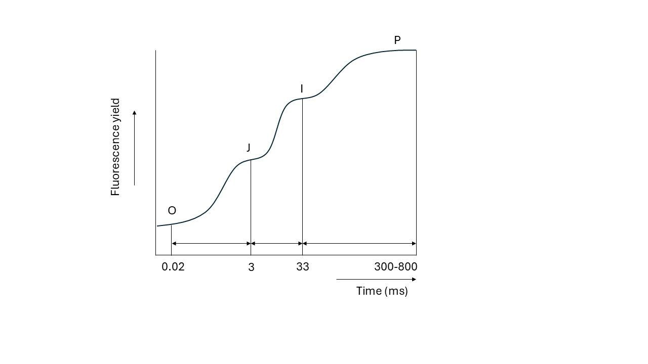
As seen, the fluorescence level rises in three steps (Strasser called it ‘triphasic kinetics’). These steps are called the J, I and P plateau. The first plateau, “J”, appears within 3 milliseconds, followed by the ‘I’ plateau at approximately 33 milliseconds. Finally, the “P” plateau marks the ‘peak’ or maximum fluorescence, usually after around 300 to 800 milliseconds.

These steps do not appear without reason; they appear because we are following the first initial charge separations (transfer of electrons from a donor to an acceptor) and reactions in the photosynthetic apparatus, which I will explain, according to Strasser’s model, in the next part.

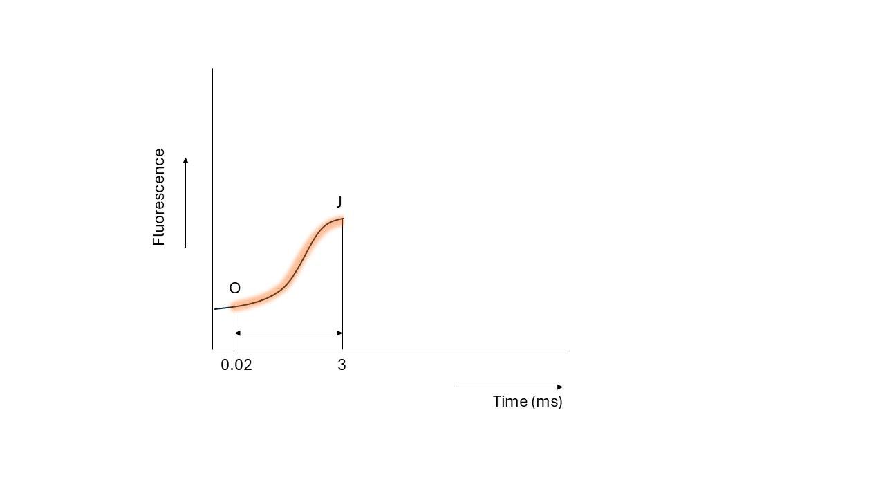
O-J step



The moment light energy is absorbed by the antenna pigments of a photosystem, almost instantly (within femtoseconds) the chlorophyll around the reaction center becomes ‘excited’ with this charge. An electron, introduced into the system by the splitting of water, can carry this energy. 
For the charged electron to move into the chain, the first electron acceptor in Photosystem II, called QA, must be in an ‘open’ state (‘free of electrons’). The moment QA accepts a charged electron, a small fraction of the excitation energy is released as fluorescence, which we detect as the minimal fluorescence, or origin fluorescence (Fo). This process happens very quickly; Fo is measured after just 0.05 milliseconds. 

When QA is ‘occupied’ by an electron, it cannot accept another one until the first electron passes to the next electron carrier, called QB. However, excitation of chlorophyll is a faster process than the passing of electrons, which means the absorbed light energy cannot enter the electron transport chain due to QA being still occupied. Because of this, the excited chlorophyll returns to its ground (uncharged) state by releasing the excess energy as fluorescence (one of the three possible fates of energy). This results in an increase in fluorescence, which is observed as the rise from O to J in the fluorescence induction curve. 

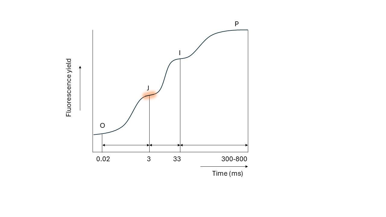
J-I step

At the time the electron is transferred from QA to QB (the second electron carrier in PSII), another electron can be accepted by QA. This means light energy can be used for photochemistry again, and as a result, less energy is released as fluorescence (remember the three possible fates of absorbed light). The movement of electrons from QA to QB therefore leads to a temporary stabilization of the fluorescence level, as the rate of QA closing equals the rate of QA reopening. This stabilization becomes visible after roughly 3 milliseconds, where fluorescence reaches a steady level, known as the J plateau. 

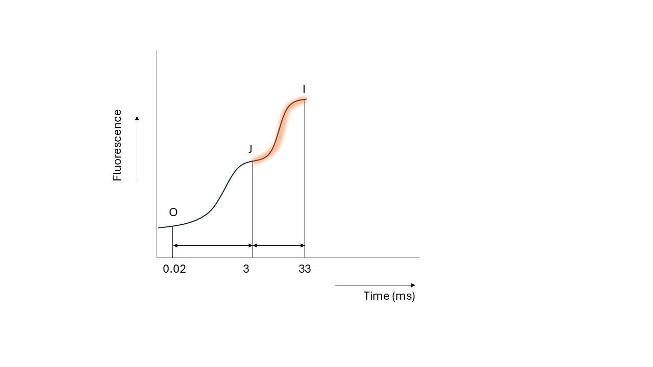
The second electron carrier, QB, requires two electrons before it passes them on to the next electron acceptor. Once QB receives a second electron from QA, it takes up two protons (H⁺) from the stroma and becomes plastoquinol (PQH₂). PQH₂ then leaves photosystem II and diffuses into the plastoquinone (PQ) pool within the thylakoid membrane.

Eventually, the cytochrome b6f complex accepts these electrons. However, cytochrome b6f can only accept and process electrons from PQH₂ at a finite rate, creating a bottleneck. 

Because of the limitations of cytochrome b6f, PQH₂ accumulates in the pool, which slows down the flow of electrons. QA cannot pass on new electrons because QB is still occupied. As a result, light energy cannot enter the electron transport chain, causing the excited chlorophyll to fall back to the ground state, releasing energy as fluorescence again. This causes the fluorescence level to rise, which is observed as the transition from J to I. 

I-P step

However, like earlier stages, PC and PSI require some time to reach full efficiency. This delay creates again a bottleneck further downstream in the chain. Under the conditions of the extreme high light intensity (during the 1 second pulse), the whole system is now saturated, meaning all electron carriers are ‘closed’ and unable to accept more electrons.

When this happens, light energy cannot be transferred into the electron transport chain and the excited chlorophyll again falls back to the ground state, releasing energy as fluorescence. This leads to the final rise in fluorescence, reaching the maximum level (Fm), observed as the P peak in the OJIP curve. 

What can we do with this?

As you can see, during the 1-second light pulse, many processes can be followed. From these plateaus and the shape of the curve, the functioning or efficiency of the system can be quantified. Strasser and his colleagues, and other researchers, created more than 25 formulas that allow us to calculate how the plant’s photosynthetic apparatus is functioning. These derived parameters range from an overall efficiency of the system to zoomed into individual processes, for instance:

• Light absorption- and trapping parameters

(antenna size, trapping flux per center, first electron acceptor efficiency)

• Reaction center parameters

(# of reaction centers per chlorophyll, # of open reaction centers, efficiency per center)

• Electron transport parameters

(Electron transport flux per center, efficiency of transport to different electron acceptors)

• Energy conversion parameters

(Dissipation flux, photochemical flux)

Stress (such as drought stress, heat stress, salt stress, or pests and diseases) have a huge effect on the functioning of the system, and therefore can be picked from these measurements. Also modes of actions of products can be quantified.

In part 2 of the OJIP blog, I will focus on the parameters that are calculated from the OJIP rise, what they mean, and summarize the effects of stress on them. 

References

• Strasser, R.J., Srivastava, A. And Govindjee (1995). Polyphasic chlorophyll a fluorescence transient in plants and cyanobacteria. Photochemistry and Photobiology 61: 32-42.

•  Strasser, R.J., Srivastava, A. And Tsimilli-Michael, M. (2000). The fluorescence transient as a tool to characterize and screen photosynthetic samples. In: Ynus, M. (Ed.) Probing Photosynthesis: Mechanisms, Regulation and Adaptation. Taylor and Francis, London: 445-483.

• Strasser, R.J., Tsimilli-Micael, M. and Srivastava, A. (2004). Analysis of the Chlorophyll a fluorescence transient. In: Papageorgiou, G.C. and Govindjee (Eds.) Chlorophyll a fluorescence: a signature of photosynthesis. Springer, Dordrecht: 321-362.

• Tsimilli-Michael, M. (2020). Revisiting JIP-test: An educative review on concepts, assumptions, approximations, definitions and terminology. PHotosynthetica 58: 275-292.